Estimating expectations with respect to high-dimensional multimodal distributions is difficult. Here we describe an implementation of Hamiltonian annealed importance sampling in TensorFlow and compare it to other annealed importance sampling implementations. This is joint work with Halil Bilgin.
Introduction
Radford Neal showed how to use annealing techniques to define importance samplers suitable for complex multimodal distributions. Sohl-Dickstein and Culpepper extended his work by demonstrating the utility of Hamiltonian dynamics for the transition kernels between the annealing distributions. We summarise these developments here.
Naive Monte Carlo expectations
A naive yet often practical way to estimate the expectation of a function $f(x)$ is simply to sample from the underlying distribution $p(x)$ and take an average:
\[\mathbb{E}_p[f(X)] \approx \hat{\mu} = \frac{1}{N} \sum_{n=1}^{N} f(X_n), \qquad X_n \sim p\]However when $f(x)$ is close to zero outside some set $\mathcal{A}$ where $\mathbb{P}(X \in \mathcal{A})$ is small, samples from $p(X)$ typically fall outside of $\mathcal{A}$ and the variance of $\hat{\mu}$ is high. Estimating the marginal likelihood (or evidence) for a model given some data $\mathcal{D}$ is a canonical example of this. In this case $f(x) = p(\mathcal{D}|x)$ is the likelihood and $p(x)$ is the prior. For many models and data the posterior will be highly concentrated around a typical set, $\mathcal{A}$, that only has small support under the prior. That is $p(\mathcal{D}|x)$ will be small for most samples from $p(x)$ and a few terms in the average will dominate, resulting in a high variance estimator.
Importance Sampling
Importance sampling (IS) is a method that can be well-suited for estimating expectations for which the naive Monte Carlo estimator has high variance. The IS estimate of the expectation is
\[\hat{\mu}_q = \frac{1}{N} \sum_{n=1}^{N} \frac{f(X_n) p(X_n)}{q(X_n)}, \qquad X_n \sim q\]where $q$ is the importance distribution and $p$ is the nominal distribution. Choosing $q=p$ gives the naive Monte Carlo estimator. A well chosen $q$ will give $\mathbb{V}[\hat{\mu}_q] < \mathbb{V}[\hat{\mu}]$. A badly chosen $q$ can give $\hat{\mu}_q$ infinite variance. The ideal $q$ is proportional to $f(x)p(x)$. However in general this is not helpful as the required normalising constant is the intractable expectation we wish to estimate in the first place.
Annealed Importance Sampling
Finding good importance distributions when $X$ is high-dimensional and/or $p$ is multimodal can be difficult. This makes the variance of $\hat{\mu}_q$ difficult to control. Annealed importance sampling (AIS) is designed to alleviate this issue. AIS produces importance weighted samples from an unnormalised target distribution $p_0$ by annealing towards it from some proposal distribution $p_N$. For example,
\[p_n(x) = p_0(x)^{\beta_n} p_N(x)^{1-\beta_n}\]where $1 = \beta_0 > \beta_1 > \dots > \beta_N = 0$. To implement AIS we must be able to
- sample from $p_N$
- evaluate each (potentially unnormalised) distribution $p_n$
- simulate a Markov transition $T_n$ for each $1 \le n \le N-1$ that leaves $p_n$ invariant
Hamiltonian Annealed Importance Sampling
Hamiltonian annealed importance sampling (HAIS) is a variant of AIS in which Hamiltonian dynamics are used to simulate the Markov transitions between the annealed distributions. An important feature is that the momentum term is partially preserved between transitions.
Examples
Log-gamma normalising constant
Unnormalised versions of well known densities are useful test cases for annealed importance samplers. If $p$ is such an unnormalised density function then its normalising constant is simply $\mathbb{E}_p[1]$ and can be estimated using AIS. This estimate can be compared against the exact value to double-check the validity of the estimate.
$X$ is said to be distributed as $\textrm{log-gamma}(\alpha, \beta)$ when $\log X \sim \Gamma(\alpha, \beta)$. The probability density function for a gamma distribution is
\(f(x; \alpha, \beta) = \frac{\beta^\alpha}{\Gamma(\alpha)} x^{\alpha-1} e^{- \beta x}\) for all $x > 0$ and any given shape $\alpha > 0$ and rate $\beta > 0$. Given a change of variables $y = \log(x)$ we have the density for a log-gamma distribution
\[f(y; \alpha, \beta) = \frac{\beta^\alpha}{\Gamma(\alpha)} e^{\alpha y - \beta e^y}\]Thus if we define our unnormalised density as $p_0(x) = e^{\alpha x - \beta e^x}$ its normalising constant is $\frac{\Gamma(\alpha)}{\beta^\alpha}$.
Running our HAIS sampler on this unnormalised density with $\alpha = 2$, $\beta = 3$
and a standard normal prior gives these samples
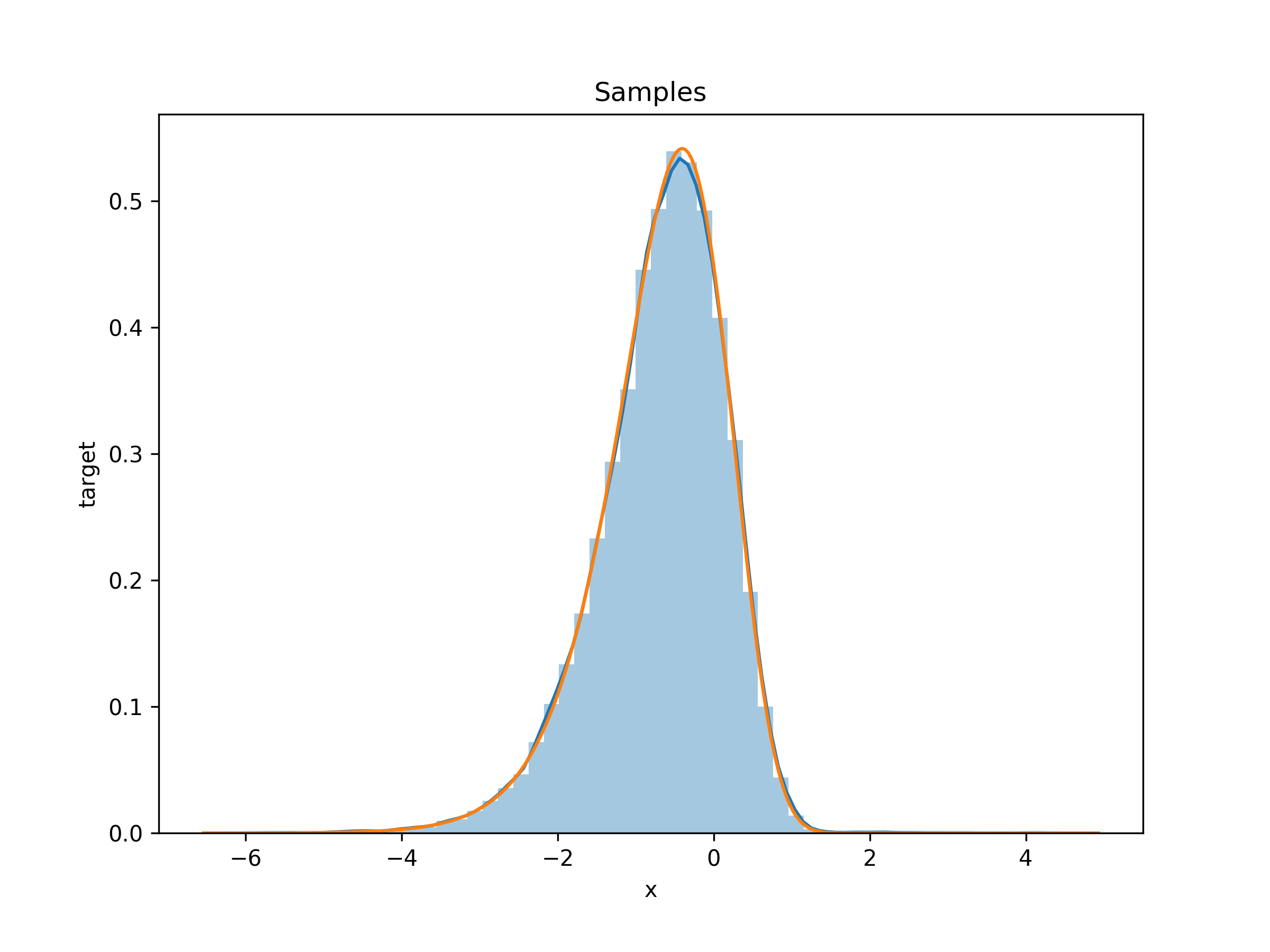 and the estimate of the log normalising constant is -2.1975 (the true value is -2.1972).
Marginal likelihood
We used our HAIS implementation to estimate the marginal log likelihood for a
latent variable model for which an analytic solution is known (model 1a from
Sohl-Dickstein and Culpepper). In the plot below we compare our HAIS estimates
with those estimated by the BayesFlow AIS sampler that is included with
TensorFlow (version 1.6). 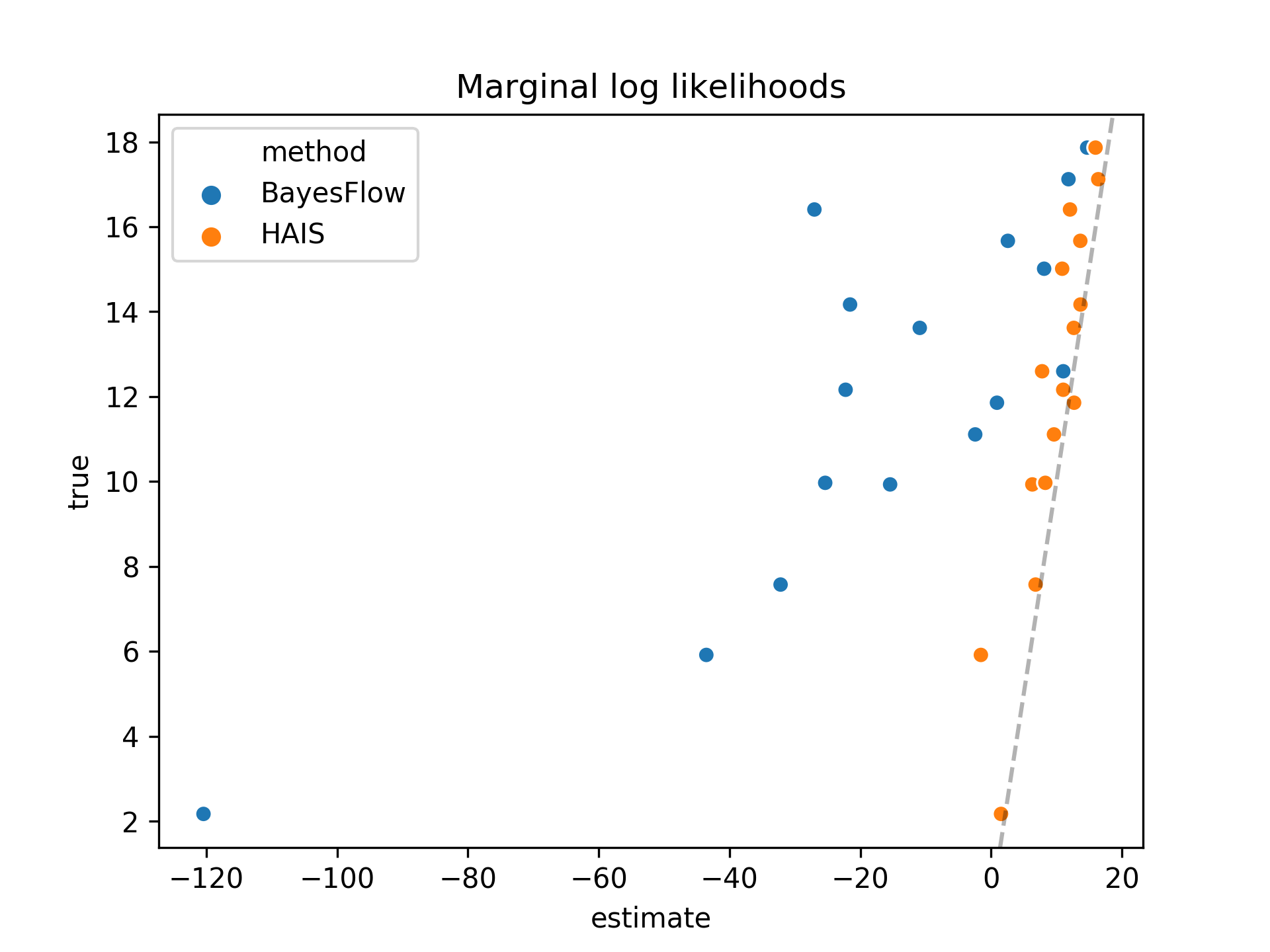 The dotted line represents
the ideal marginal log likelihood estimates. We see our estimates are much
closer to these true values.
The dotted line represents
the ideal marginal log likelihood estimates. We see our estimates are much
closer to these true values.
Implementation
Our implementation is available under a MIT license. Test scripts to generate the figures in this post are also available.